Dynamic Scoring Made Simple

Key Findings

• Dynamic scoring is a tool to give members of Congress the information they need to evaluate the tradeoffs in taxA tax is a mandatory payment or charge collected by local, state, and national governments from individuals or businesses to cover the costs of general government services, goods, and activities. policy changes.
• Dynamic scoringDynamic scoring estimates the effect of tax changes on key economic factors, such as jobs, wages, investment, federal revenue, and GDP. It is a tool policymakers can use to differentiate between tax changes that look similar using conventional scoring but have vastly different effects on economic growth. provides an estimate of the effect of tax changes on jobs, wages, investment, federal revenue, and the overall size of the economy.
• Using dynamic scoring, policymakers can differentiate between policies that look similar using conventional scoring methods, but have vastly different effects on economic growth under dynamic scoring.
• For example—using Tax Foundation’s Taxes and Growth model—we find that five tax change with the same static revenue cost can have vastly different effects on GDP, investment, jobs, and federal revenue—ranging from virtually no change in GDP to an increase of over 5 percent.
• The use of dynamic scoring is crucial to ensure that comprehensive tax reform grows the economy and meets revenue expectations.

Introduction

The new House-passed rule requiring dynamic scoring of substantive tax legislation has brought criticism from all quarters of Washington—lawmakers, pundits, and think tank types. To many, dynamic scoring is seen as a smokescreen to justify tax cuts without having to pay for them. To others, dynamic scoring is an attempt by the majority to impose a particular ideology on the nonpartisan Congressional Budget Office. Still others say that there is too much disagreement among economists about assumptions to perform dynamic scoring on a routine basis.

In reality, dynamic scoring is no different than conventional scoring; it is a tool for giving members of Congress information they need to make decisions about tax policy. However, conventional scoring methods provide them a very one-dimensional perspective about the effects of tax changes. By contrast, dynamic scoring gives lawmakers three-dimensional information they can use to understand the effects of tax policies on a complex, multi-dimensional U.S. economy.

With this 360 degree information, lawmakers can differentiate between policies that might look similar using conventional methods and select policies that create economic growth and avoid policies that might harm growth.

A good way to illustrate the benefits of dynamic scoring is to contrast the macroeconomic effects of various tax policies that all have the same score using conventional methods. Tax Foundation economists used our Taxes and Growth (TAG) model to simulate the macroeconomic effects of five different tax cuts and five different tax increases; with each set of policies having the same static score using conventional methods.

The results of these simulations clearly show that tax policies that may appear to have the same cost on paper can have vastly different effects on GDP, investment, jobs, and, ultimately, on federal revenues. This exercise shows that if lawmakers are serious about reforming the tax system in a way that maximizes economic growth, dynamic scoring must be a part of that process.

A Primer: How the Taxes and Growth (TAG) Dynamic Tax Model Works

In economic jargon, the Tax Foundation’s dynamic tax model is considered a mainstream Neoclassical Growth Model. What this means is that the model is designed to isolate and measure the effects of tax changes on the cost of capital and on the cost of labor. Once these costs are calculated, the model can then simulate the effects of the tax changes on key economic factors, such as GDP, investment, and jobs, as well as important factors in the fiscal debate, such as federal revenues.

Under a neoclassical view of the economy, the willingness of people to deploy capital and to work more are the two main drivers of economic growth. Changes in the cost of capital and in the cost of labor determine the size of the capital stock in the economy and the supply of labor. The degree to which the capital stock and the labor supply expand or contract determines the level of output and income in the economy.

Taxes are an important determinant of not only how much people are willing to invest in new plant and equipment, but where they decide to locate that capital. Taxes factor into people’s decisions to join the workforce and determine how much they work.

While both capital and labor are affected by changes in tax policy, empirical evidence clearly shows that capital is far more sensitive to changes in tax policy than is labor, so changes in the taxation of capital have a far bigger effect on the economy than do changes in the taxation of the labor.

A key reason for this is that capital is far more mobile than labor. Capital can move quickly from jurisdiction to jurisdiction in search of lower tax costs (say, from the U.S. to Ireland), but it is far more difficult for workers to move their families from state to state, or even to another country, to lower their tax bills.

The Two Main Components of the TAG Model

The Taxes and Growth model is comprised of two main components—a tax simulator and a macroeconomic model.

The tax simulator can be thought of as a supersized TurboTax for the entire population of taxpayers. It computes the effects of policy changes on the marginal individual income taxAn individual income tax (or personal income tax) is levied on the wages, salaries, investments, or other forms of income an individual or household earns. The U.S. imposes a progressive income tax where rates increase with income. The Federal Income Tax was established in 1913 with the ratification of the 16th Amendment. Though barely 100 years old, individual income taxes are the largest source of tax revenue in the U.S. rates paid by taxpayers in all income groups. When this calculator is utilized alone, it generates most of the “static” results from the model.

This part of the model draws from an extensive series of IRS datasets beginning in 1965 and extending through 2011. Each dataset contains roughly 100,000 to 150,000 sample tax returns representing all of the individual tax returns filed that year. The model’s ability to access IRS datasets over time makes historical comparisons possible.^[1] This data has also been projected forward through 2025 to allow the model to make forward-looking estimates through the end of the ten-year budget window.

The companion to the simulator is the dynamic macroeconomic model, which computes changes to the returns to capital—or what economists call the “service price” of capital—as well as changes to the labor supply. This side of the model is fueled by data from the 1950s through the present, including: tax parameters, National Income and Product Account (NIPA) data, and depreciationDepreciation is a measurement of the “useful life” of a business asset, such as machinery or a factory, to determine the multiyear period over which the cost of that asset can be deducted from taxable income. Instead of allowing businesses to deduct the cost of investments immediately (i.e., full expensing), depreciation requires deductions to be taken over time, reducing their value and discouraging investment. schedules. This data is also projected out through 2025.

These two components of the model work together to calculate the dynamic effects of tax changes. From these calculations the model generates estimates of the effect of tax changes on key economic factors such as GDP, capital stocks, wage rates, jobs, and hours worked. To inform the policy debate, the model also produces both dynamic and static estimates of changes in federal revenue and distributional effects.

Let’s look at some results generated by the model.

Comparing the Dynamic Effects of Five Static Tax Cuts

Intuitively, everyone understands that no two tax changes affect the economy the same way. Tax Foundation economists tested this intuition by simulating the macroeconomic effects of five different illustrative tax cuts with our TAG model. Each of these different policies had a conventional, or “static,” revenue cost of $72 billion annually.

These five policies include:

• The creation of a new $1,000 per-child tax creditA tax credit is a provision that reduces a taxpayer’s final tax bill, dollar-for-dollar. A tax credit differs from deductions and exemptions, which reduce taxable income, rather than the taxpayer’s tax bill directly. with no upper income cap;^[2]
• Cutting the tax rate in the 10 percent tax bracketA tax bracket is the range of incomes taxed at given rates, which typically differ depending on filing status. In a progressive individual or corporate income tax system, rates rise as income increases. There are seven federal individual income tax brackets; the federal corporate income tax system is flat. to 3.5 percent;
• Cutting the rates in the top three individual income tax brackets (33, 35, and 39.6 percent) to 29.2 percent;
• Cutting the corporate income taxA corporate income tax (CIT) is levied by federal and state governments on business profits. Many companies are not subject to the CIT because they are taxed as pass-through businesses, with income reportable under the individual income tax. rate from 35 percent to 24 percent;
• Moving from the current “accelerated” depreciation system (MACRS) to full expensingFull expensing allows businesses to immediately deduct the full cost of certain investments in new or improved technology, equipment, or buildings. It alleviates a bias in the tax code and incentivizes companies to invest more, which, in the long run, raises worker productivity, boosts wages, and creates more jobs. for all capital investments, including machinery and structures.

As Chart 1 illustrates, a new $1,000 per child tax credit produces virtually no growth (for simplicity we rounded the results in hundredths of a percent to zero). The reason for this lack of growth is that a child credit is primarily a lump-sum windfall for taxpayers; it does not reduce the cost of labor nor improve the marginal incentives to work more. Indeed, some have argued that a generous enough child credit could actually encourage one spouse to leave the workforce and stay home with the children.

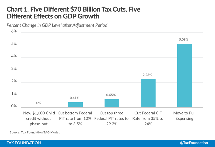
On the other hand, the model estimates that cutting the tax rate in the lowest personal income tax bracket from 10 percent to 3.5 percent boosts the level of GDP by a modest 0.41 percent. While the lower first bracket does cut the tax owed by all taxpayers, it does not reduce the tax on additional income for people whose earnings reach higher brackets, thus it provides little marginal incentives for people to join the workforce or to work longer hours. As a result, it has a small impact on the economy.

By contrast, lowering the top individual income tax brackets has a larger effect on improving incentives to work and invest—especially for entrepreneurs and pass-through businessA pass-through business is a sole proprietorship, partnership, or S corporation that is not subject to the corporate income tax; instead, this business reports its income on the individual income tax returns of the owners and is taxed at individual income tax rates. owners. As a result, these rate cuts increase the level of GDP by 0.65 percent.

Since capital is more sensitive to tax changes than is labor, the model predicts that cutting the corporate income tax rate from 35 percent to 24 percent would produce nearly four-times as much growth—indeed, boosting the level of GDP by 2.26 percent at the end of the adjustment period.

Moreover, the model shows that moving to full expensing for all equipment and buildings would achieve even greater growth, raising the level of GDP by more than 5 percent—twice as much as is achieved by cutting the corporate tax rate. Why? Because expensing dramatically cuts the cost of capital for new plant and equipment—spurring people to create more of it—whereas cutting the corporate rate benefits new and old investments alike, losing some of its punch in providing a sort of windfall for old investments, with only a portion of its power directed at adding more capital.

Now, let’s look at these effects within the context of federal revenue estimates.

Comparing the Effect of Tax Cuts on Federal Revenues

Naturally, larger economies generate more tax revenues. Since the five tax cut plans generate different levels of GDP, their “feedback” effect on federal revenues will vary considerably. In Chart 2, we show the GDP effects of these five different tax cuts in dollar terms (as opposed to the percentages in Chart 1), and compare these results against both the static revenue estimates and the dynamic results generated by the growth effects associated with each tax cut plan. This is where the value of dynamic scoring to the budget process is most apparent.

Not All Tax Cuts Pay for Themselves: The Economic Effects of Tax Changes on Labor

Like all of the five tax cuts modeled, the static revenue estimate for the child credit is a loss of $72 billion to the Treasury. Because this tax cut produces virtually no economic growth, there is no extra revenue feedback from the policy, and so it also loses $72 billion on a dynamic basis.

The individual rate cuts do produce modest economic growth and, thus, have modest revenue feedbacks. So each of these polices lose slightly less on a dynamic basis than is estimated on a static basis. For example, cutting the lowest tax bracket generates $68 billion in additional GDP. When the TAG model accounts for the modest feedback effect from this new growth, it finds that the policy costs about 20 percent less on a dynamic basis than was estimated on a static basis (-$56 billion versus -$72 billion).

Meanwhile, the plan to cut the top brackets generates $107 billion in higher GDP and, due to the feedback effects of this new growth, the plan costs about one-third less than the static cost (-$48 billion versus -$72 billion).

These three examples should clearly illustrate to both supporters and detractors of dynamic scoring that the notion that all tax cuts pay for themselves has been quite oversold. But if lawmakers are going to make smarter tax policy, it is important for them to understand the degree to which different policies generate different feedback effects on federal revenues. This is especially true if revenue neutrality is a requirement. The revenue feedback from different policies will necessitate different amounts of offsets for the plans to remain revenue neutral.

The Economic Effects of Tax Changes on Capital

The above policies primarily affect the cost of labor, which we know is not as sensitive to tax changes as is the cost of capital. The TAG model shows us that there are a very select group of tax cuts that can “pay for themselves” over the long-term by recouping their projected static revenue costs because they so dramatically reduce the cost of capital and, thus, generate substantial economic growth. As Chart 2 illustrates, cutting the corporate tax rate to 24 percent and moving to full expensing for all capital expenditures are select examples of policies that can generate more new tax revenues than they lose over time.

The TAG model estimates that cutting the corporate tax rate to 24 percent would boost the level of GDP by nearly $370 billion. The resulting feedback from this new growth, in turn, would generate an additional $11 billion in federal revenues by the end of the adjustment period—roughly 10 years out. However, it is important to note that the policy would lose revenues during the early years of the program as the economy adjusts to the new tax rates.

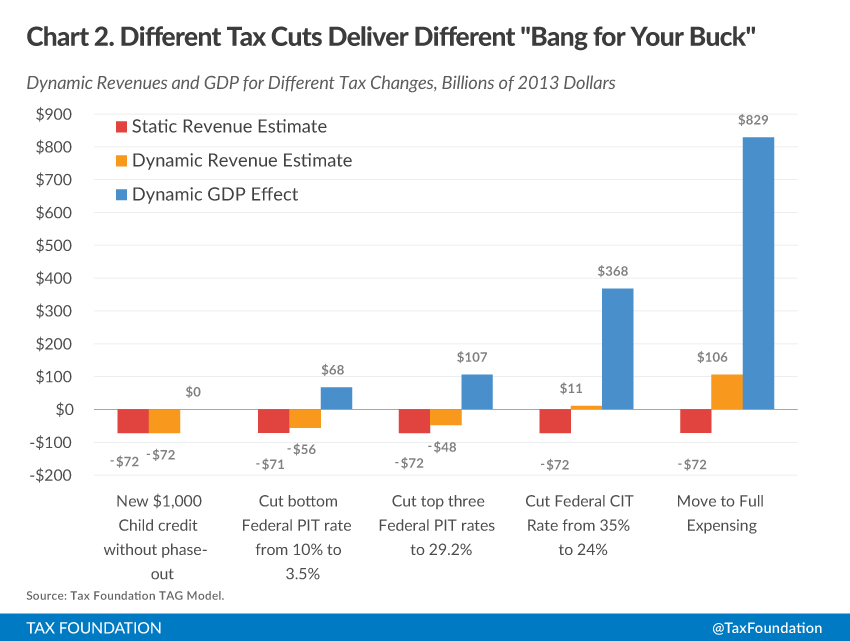
Chart 2 shows that the move to full expensing would produce even more growth—more than $800 billion in higher GDP. As a result, the feedback effect from this policy would generate $108 billion in additional federal revenue each year after all adjustments. So not only would the economy benefit from this policy, but the federal Treasury would eventually benefit as well.

Different Tax Increases Also Generate Different Results

It is only natural that if all tax cuts don’t have the same effect on the economy, then neither do all tax increases. Should members of Congress decide to raise taxes to reduce the deficit or to finance new spending programs, it is very important that they know which tax hikes are going to deliver the maximum amount of new revenues with the least harm to the economy. Otherwise, they risk choosing policies that will so reduce the level of GDP that they ultimately deliver less than the anticipated amount of revenues, resulting in higher deficits.

This is another added value of dynamic scoring. It can give policymakers the information they need to make a reasoned decisions about the tradeoff between the economy and federal tax revenues. Conventional scoring cannot give them that information.

Using the TAG model, Tax Foundation economists modeled five different illustrative tax increases, all with a static scoring of about $32 billion. The dynamic results of these policies are as varied as the dynamic results from the tax cuts.

The five tax increases included:

• Lengthening depreciation lives by moving from our current accelerated depreciation system (MACRS) to the straight line Alternative Depreciation System (ADS);
• Raising the corporate income tax rate from 35 percent to nearly 40 percent (39.8);
• Raising the rate of the top individual income tax bracket from 39.6 percent to 44.5 percent;
• Raising the rate of the bottom individual income tax bracket from 10 percent to 12.5 percent;
• Disallowing half of the state and local tax deductionA tax deduction is a provision that reduces taxable income. A standard deduction is a single deduction at a fixed amount. Itemized deductions are popular among higher-income taxpayers who often have significant deductible expenses, such as state and local taxes paid, mortgage interest, and charitable contributions. .

As Chart 3 shows, of these five policy options, moving from our current MACRS depreciation system to ADS has the biggest impact on GDP because it has the biggest effect on the cost of capital. This policy reduces the level of GDP in the long-run by nearly 2 percent because it severely raises the cost of capital, which, in turn, depresses the quantity of capital employed in the economy.

Similarly, although in a less dramatic fashion, raising the corporate tax rate from 35 percent to nearly 40 percent would lower GDP by more than 1 percent. The impact on the economy from raising the corporate tax rate is less severe than lengthening depreciation lives because it effects old capital as well as new investment. Investors and businesses cannot change the past, so they tend to be a captured tax baseThe tax base is the total amount of income, property, assets, consumption, transactions, or other economic activity subject to taxation by a tax authority. A narrow tax base is non-neutral and inefficient. A broad tax base reduces tax administration costs and allows more revenue to be raised at lower rates. . Since their investments are already in place, new taxes on those profits will have relatively little effect on their behavior.

Since labor is less sensitive to higher taxes than capital, raising individual income tax rates has less of an impact on GDP than does increasing the corporate income tax. Chart 3 shows that raising the top individual income tax rate from 39.6 percent to more than 44 percent would lower GDP by 0.33 percent because it would impact the marginal decisions to work and invest by high-income people, who tend to be entrepreneurs, investors, and owners of pass-through businesses.

By contrast, raising the 10 percent tax bracket to 12.5 percent would impact a broader swath of taxpayers—because even wealthy taxpayers pay the lowest rate on their first dollars of income—but it would have a smaller impact on GDP because it affects fewer decisions of people to enter the workforce or to work longer hours.

For example, union workers are not likely to reduce their overtime hours if the lowest bracket is raised to 12.5 percent because that rate may only affect their base pay. But they might stop working overtime if the 15 or 25 percent tax bracket rates were lifted, because their overtime pay would be subject to those higher rates. Thus, the model estimates that this policy would lower GDP in the long-run by 0.21 percent.

The TAG model shows that of these five illustrations, the tax hike with the least effect on GDP is disallowing half of the state and local tax deduction. While eliminating a tax deduction certainly raises a family’s effective tax rate, it has less of an impact on work incentives than a pure rate increase and, thus, has a smaller impact on GDP. Chart 3 shows that this tax increase would lower the level of GDP by 0.16 percent.

Now let’s look at these GDP effects within the context of the static and dynamic revenue effects.

Different Tax Increases Have Different Dynamic Revenue Effects

In Chart 4, we can see that each of these five tax measures is estimated on a static basis to cost the Treasury around $32 billion. However, we can also see that there is a large tradeoff between these expected revenues and lower GDP. And lower GDP means lower incomes for people at all income levels.

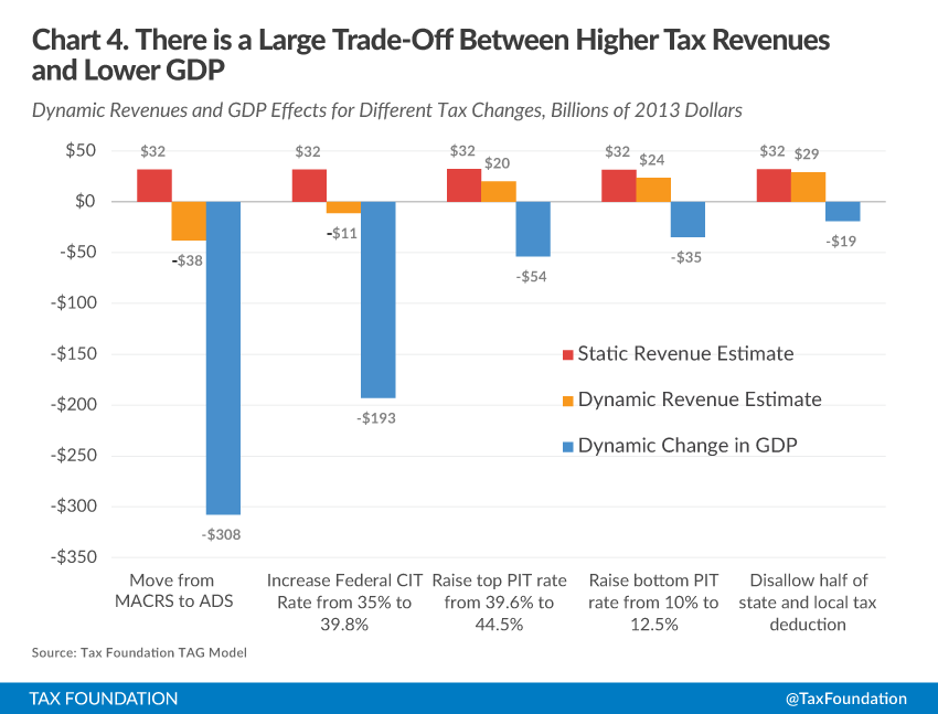
The most extreme of these examples is the move from MACRS to ADS, which is estimated to reduce GDP by more than $300 billion. Thus, for every dollar that the policy is expected to raise on a static basis, it would reduce GDP (and, thus incomes) by about $10. And because the reduction in GDP is so large, the policy ends up losing more revenues on a dynamic basis (-$38 billion) than it is estimated to gain on a static one.

Although not as extreme, raising the corporate income tax rate would lower GDP (and incomes) by $193 billion, or roughly $6 for every $1 that it is expected to raise on a static basis. The model shows that this policy would also lose revenue (-$11 billion) after we account for the economic effects of the policy.

In contrast to these examples, the TAG model finds that increasing individual tax rates will reduce GDP, but can generate new tax revenues—though not as much as is estimated on a static basis.

Chart 4 shows that raising the top income tax bracket to 44.5 percent would lower the level of GDP by $54 billion. As a result of this lower level of GDP, the policy would raise $20 billion in new revenues, or only two-thirds (62.5 percent) of the static estimate.

The revenue gain from lifting the lowest income tax bracket would be better, but still at a cost to GDP of $35 billion. The lower income levels would generate $24 billion in new tax revenues, or 75 percent of what the policy would be expected to raise on a static basis.

It should be noted here that the true cost to the economy of these policies is more than just the loss in GDP. In the case of raising the top income tax rates, we must add the $20 billion in new tax revenues to the $54 billion in lower GDP. This brings the total cost to the private sector to $74 billion—which is more than twice what the policy was expected to raise in revenues on a static basis. And even though lifting the lowest income tax bracket would generate 75 percent of the static estimate in new revenues, the cost to people in lost income (GDP) is more than how much federal revenue the policy was expected to generate on a static basis.

Finally, since disallowing a portion of the state and local tax deduction would have the least negative impact on GDP, it would actually come closest to raising as much revenue on a dynamic basis as it would be expected to do on a static one. Chart 4 shows that once the full economic effects of the policy were taken into account, it would generate $29 billion in new revenues, or 90 percent of the expected static amount.

What Do These Results Tell Us About Comprehensive Reform Plans?

It is critically important that policymakers understand the economic effects of individual policies so that when they combine these pieces into a comprehensive tax reform plan, they have a good idea of which parts will create growth and which parts will not—especially which parts might actually neutralize the growth effects of other pieces of the overall plan.

With the lessons of the ten previous examples in mind, let’s look at the dynamic effects of more comprehensive and ambitious tax plans.

Here, we contrast the dynamic effects of a stylized consumption taxA consumption tax is typically levied on the purchase of goods or services and is paid directly or indirectly by the consumer in the form of retail sales taxes, excise taxes, tariffs, value-added taxes (VAT), or an income tax where all savings is tax-deductible. versus a stylized high-tax plan. Both plans are intended to be revenue neutral.

The consumption plan is a modified “X-Tax.” Basically, this is a variant of a flat taxAn income tax is referred to as a “flat tax” when all taxable income is subject to the same tax rate, regardless of income level or assets. or cash flow tax with graduated rates for individuals, with the top bracket being set at 35 percent. Income from saving would not be taxes at the personal level. All income from investments would be taxed at a uniform business tax rate of 35 percent. The tax rate for corporate income would also be set at 35 percent. Businesses would get full expensing while individuals would get a healthy personal exemption.

The high-tax income tax plan would boost the top individual tax rate to 50 percent, and it would treat capital gains and dividend income as ordinary income. Any new revenues from the plan would fund generous tax credits for low- and middle-income taxpayers.

As Chart 5 shows, the differences in the economic effects of these plans could not be greater.

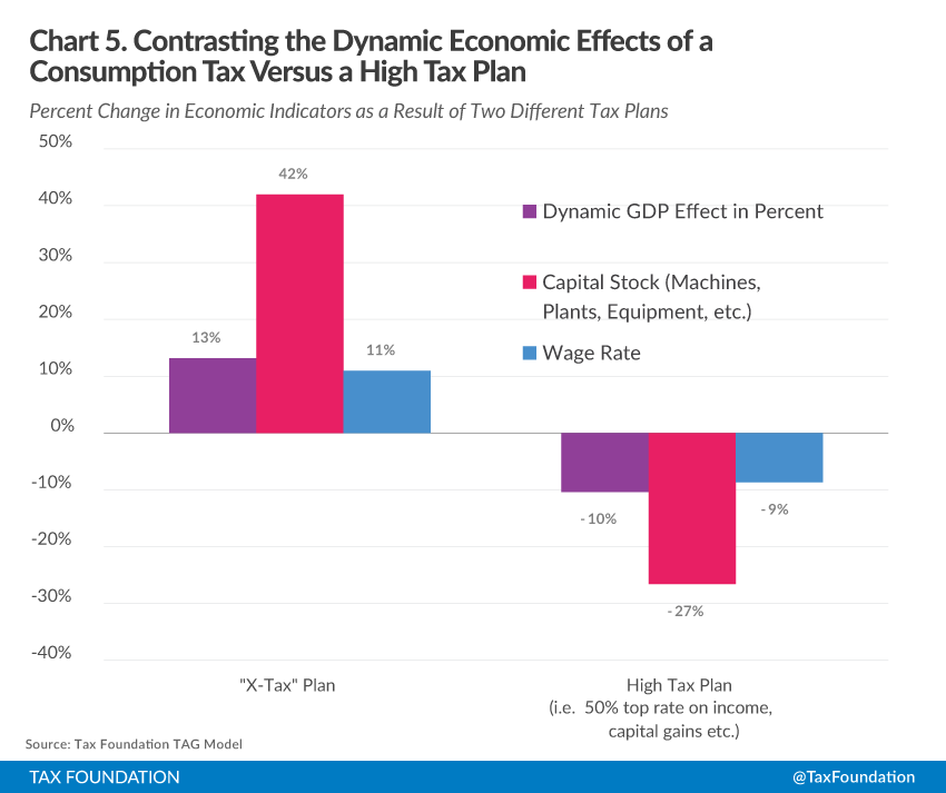
The TAG model estimates that the X-Tax plan—which would dramatically lower the cost of capital and the cost of labor—would boost GDP by 13 percent, business stocks by 42 percent, and wages by 11 percent.

By contrast, the high-tax plan—which would increase the cost of capital and decrease the incentives to work—would reduce GDP by 10 percent, business stocks by 27 percent, and wages by 9 percent.

Chart 6 puts these GDP effects in dollar terms and compares them to the resulting impact on federal revenues. We can see that the X-tax plan would boost GDP by more than $2.1 trillion per year at the end of the adjustment period. In turn, this would boost federal revenues by more than $400 billion.

The high-tax plan has the opposite effect. GDP would fall by nearly $1.7 trillion per year, which, in turn, would reduce federal revenues by about $180 billion per year. If low- and middle-income tax credits were increased based on the revenues that fail to materialize, the federal budget deficit would necessarily increase. In fact, unless the government cut its spending in line with the fall in its revenues, the budget deficit would grow.

Studies by the OECD and others have shown that there is a tradeoff between progressivity and economic growth, and these simulations clearly shows how much.

The Dynamics of Distributional Tables

Another advantage of dynamic models is the second layer of information it provides about the distributional impact of tax changes on families in different income groups. Conventional analysis displays only the legal incidence of a tax change. In other words, how does the policy affect the income of those people who write the check to the IRS? Does the policy raise their after-tax incomeAfter-tax income is the net amount of income available to invest, save, or consume after federal, state, and withholding taxes have been applied—your disposable income. Companies and, to a lesser extent, individuals, make economic decisions in light of how they can best maximize their earnings. or reduce it?

But as we have seen, tax changes can have a significant effect on the level of GDP, investment, wages, and jobs. Generally speaking, tax changes that boost GDP will lead to higher incomes for everyone, whereas tax policies that lower GDP will lead to lower incomes. Thus, tax changes can impact the living standards of people beyond those who actually write the check to the IRS. Failing to account for these effects makes conventional scoring very one-dimensional.

Dynamic analysis measures the changes in taxpayer incomes after taking into account how tax changes impact the economy. A good example of this three-dimensional approach to distributional analysis can be seen with the corporate income tax.

Table 1 contrasts the two approaches to measuring the effects of a corporate tax cut on individual taxpayers. Under conventional scoring, a corporate tax cut would be seen as providing little or no benefit to individual taxpayers. If it did, it would show only the benefits that would accrue to shareholders.

However, a dynamic model, such as the Tax Foundation’s TAG model, traces the economic growth benefits of a corporate tax rate cut through the growth in investment, wages, and hours worked to the higher after-tax incomes of families at all income levels. As Table 1 illustrates, cutting the corporate tax rate to 25 percent can boost the after-tax incomes of all taxpayers by 1.76 percent, with the benefits being spread up and down the income scale.

Conclusion

Despite the recent criticism of dynamic scoring, Members of Congress are being ill-served by the current conventional, or “static,” scoring method, which provides lawmakers a very one-dimensional picture of the effects of tax changes.

If Members of Congress are to make sound tax decisions that impact today’s complex, global economy, they need the three-dimensional perspective that is only possible with dynamic scoring.

As we have seen, five different tax policies that conventional scoring would say have the same cost to the U.S. Treasury, can have very different effects on the economy and, ultimately, on federal revenues when those effects are accounted for.

The primary goal of comprehensive tax reform is economic growth. Conventional scoring treats this process as an exercise in arithmetic, whereas dynamic scoring makes the process an exercise in economics. The well-being of the American people is at stake. It is critically important that lawmakers make the right choices that lift everyone’s standards of living. Only dynamic scoring can help them do that.

---

Share